English /
  Japanese
 English / Japanese
Thank you for using our product. This document guides you through R AnalyticFlow 3 (RAF3). Feedbacks are greatly appreciated: please mail to rflow-support at ef-prime.com.
Note
Some of the contents may be based on development version of the software.
Download an appropriate package for your system. RAF3 is available for Windows (64/32bit), Mac OS X and Linux.
Follow the instructions below appropriate for your system.
- Install R. Visit CRAN (The Comprehensive R Archive Network) mirrors to obtain R.
- Install RAF3. Launch the installer and follow the instructions.
Double-click on the application shortcut icon
to launch RAF3.
- Install Java 8 JDK (Java Development Kit). Visit Oracle's website to obtain JDK.
- Install R. Visit CRAN (The Comprehensive R Archive Network) mirrors to obtain R.
- Install rJava package. Launch R and execute:
install.packages("rJava")- Open the zip archive of RAF3 and drag & drop the application icon into your Applications folder.
Click on the application icon
to launch RAF3.
Upgrading to El Capitan
After upgrading to OS X 10.11 (El Capitan) you may need to re-install R before launching R AnalyticFlow.
- Install Java 8 JDK (Java Development Kit). Visit Oracle's website to obtain JDK.
- Install R. Visit CRAN (The Comprehensive R Archive Network) mirrors to obtain R.
- Configure R. Execute the following command on the console:
sudo R CMD javareconf- Install rJava package. Launch R and execute:
install.packages(c("rJava", "JavaGD"))- Extract the tar.gz archive of RAF3:
tar xzvf RAnalyticFlow_Linux_<VERSION>.tar.gzIf
javareconfdoes not work well,JAVA_HOMEmay need to be specified. Example:sudo R CMD javareconf JAVA_HOME=/usr/java/defaultA directory named
RAnalyticFlow_<VERSION>will be created after the process above. Enter into this directory and execute the following command to run RAF3:./rflow &
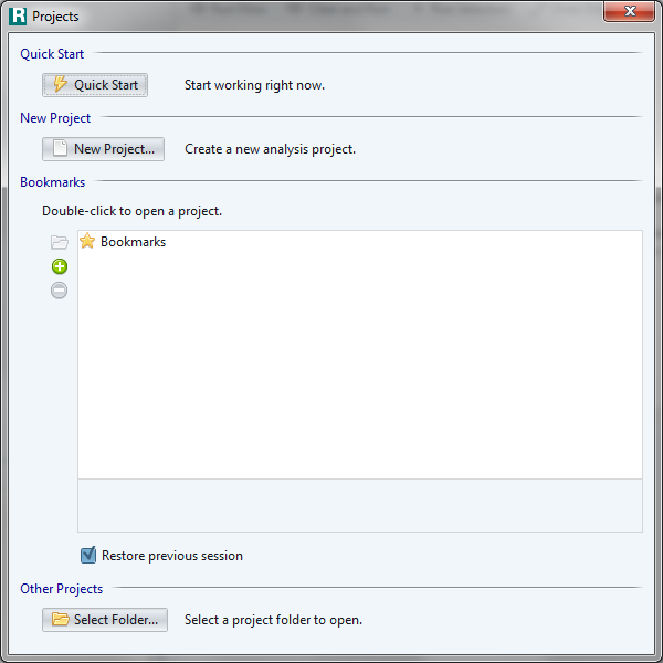
By launching RAF3 you will see the following dialog after the initial setup. Click on Quick Start button to start your work.
You will be asked to install some of required packages (
rJava,JavaGDandcodetools) if missing.
An analysis flow represents workflow of data analysis. You can create, edit, save and load an analysis flow.
Let's see an example to understand the concept of analysis flow. Click on Help > Tutorial > 1. Introduction from the menu.
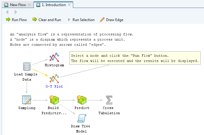
Each node (icon) represents a process of data analysis and contains corresponding R scripts. You can run the flow to execute these processes in order.
Select the X-Y Plot node and click on the Run Flow button to see the result.
You can also run a single node by Run Selection button. Try running Histogram node for example.
Notes for RAF2 users
In RAF3 you can load any
.rflowfile created with RAF2 (with new look-and-feel). New features in RAF3 will be introduced later.If you often use keyboard shortcuts, please note that Ctrl + R now works as Run Node, rather than Run Flow as in RAF2. To Run Flow in RAF3, use Ctrl + Shift + R instead.
you can edit multiple analysis flow files in RAF3. In the figure above you can see two flows, New Flow and 1. Introduction, at the same time.
Later we will introduce the concept of project to manage resources like flow files, data, documents and other resources.
Finally close the window to quit the program.
Now we are going to introduce how to analyze data, and to create analysis flow with RAF3. Launch RAF3 and follow the instructions below in Quick Start mode.
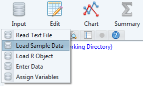
Basically data analysis is done using Analysis Modules on RAF3. Click on the Input icon on the tool bar and select Load Sample Data.
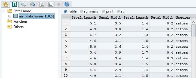
Then you can see the dialog below. Enter iris in the Data text box and you will see the preview of the result.
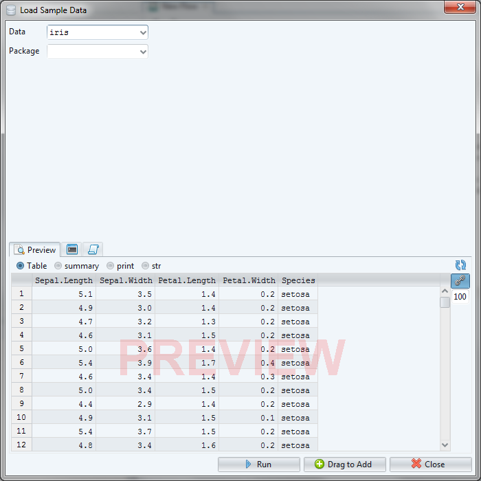
The preview is generated in a dedicated environment not to affect the current workspace. In RAF3 you can see this preview in various situations. Please be aware that the preview is not always identical to the actual result, since it is usually generated with only a small subset of data.
Click on Run button to actually load the data. Then the PREVIEW sign disappears to indicate this is the actual result. It reports no error and seems successful this time.
Let's leave this operation in an analysis flow. Drag Drag to Add button and drop on the working flow.
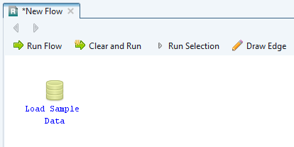
Then a corresponding icon is added in the flow. This icon is called a node.
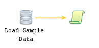
You can also add a node by drag and drop operation of a module icon. For example click on the Script on the tool bar, and drag the R Script icon and drop it into a blank space of a flow.
Try dragging the above R Script node on the Load Sample Data node. Nodes are connected by an arrow, which is called an edge.
The following are alternative ways to draw an edge:
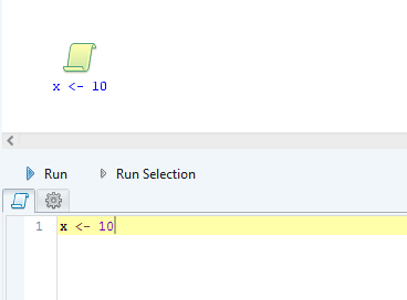
R script node is a node where you can write R script directly. To create an R script node, drag and drop R Script from Script on the tool bar.
You can also double-click on a blank space of analysis flow to create an R script node.
Lots of analysis modules can reflect your selection of objects.
Let's see an example. Select the iris object in the R Object tab as the figure below:
Next click on the Output on the tool bar and select Write Text File icon. This module can be used to output a data.frame object to a plain text file.
Then you will see the dialog below:
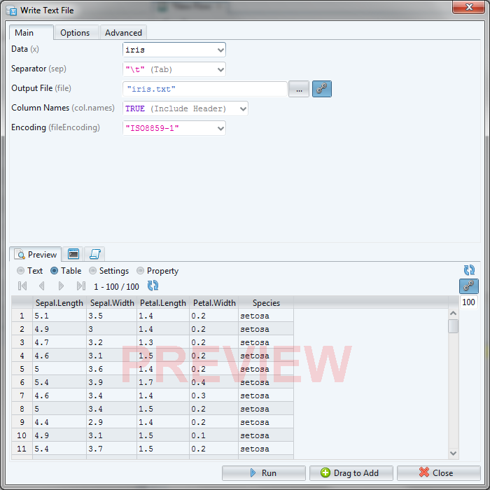
Here the name of object (iris as Object) has been automatically entered according to your selection of the object. The name of output file (File) is iris.txt by default. Parameters such as Separator and Column Names have also been set automatically but you can change them as you like.
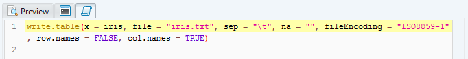
The module generates appropriate R code according to these selection of parameters. Select Script tab to review the code generated:
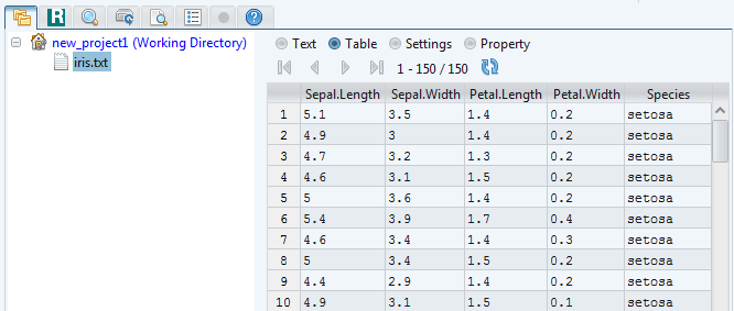
Then Run to execute the code and try Drag to Add.
You can follow the same procedure when loading a text file to R's data.frame object. Select iris.txt on the File tab first:
Next click on the Input on the tool bar and select Read Text File icon:
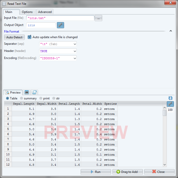
Then you can see that iris.txt is selected as the input, with auto-detected parameters.
RAF3 has a simple system for project management. It is a file-based system which can be used with other management systems including Git or RStudio.
To create a new project in RAF3, choose a project home directory first. It can be any directory including existing RStudio project directory. By default project home is also used as the working directory of R session.
In Quick Start mode you can start your work without configuring a project. In the background a temporary directory is created and it is used as the project home.
This temporary home directory will be deleted when you quit the program or start another project (including a new Quick Start session), until you save the project beforehand.
To save the project, click on  button on the tool bar. Enter the name of a directory to use as the new project home. All the data including analysis flows are moved to the new project home directory.
Launch RAF3 to show the following dialog. If it's already running, click on the  button on the toolbar.
Click on New Project... button. Then you will be asked the Project Name and its Location. In this example the project name is MyProject, and the location is C:\\Users\user\Documents\RAnalyticFlow\MyProject.
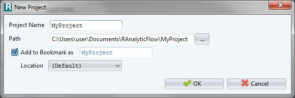
Click on OK. Then the new project has been made and you can start working on it.
Project Home is a directory where you will store any information about the project. A typical data analysis project consists of data, process (analysis flow / scripts) and documents. It may also contain binary files, property files or meta data files (.git directory for example).
The following diagram is an example of project home directory:
* Project Home/
    |
    +-- (analysis flow files)
    |
    +-- (data files, documents, scripts, etc.)
    |
    +-- .afp/
        |
        +-- (project information files)
.afp is a (hidden) directory which contains internal information about the project. It may be invisible depending on your system settings. This directory is not intended to be edited by users, so please be careful if you touch it.
It is not always a good practice to store all resources in a single directory. As a common case you may want to store data files in a remote server while you are working on your local machine.
To support such cases a link to a directory or file can be included in a project. The following diagram shows you the concept:
* (Link to) some directory/
    |
    +-- ...

* (Link to) some file
These links are shown along with the project home directory. See the figure below for example:
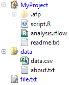
Here data directory and file.txt are not in the project home, but can be accessed easily by links.
There are two ways to create a link:
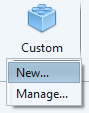
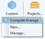
In RAF3 you can create your own module. To create a new custom module, click on Custom on the toolbar and select New....
First specify a function that you want to build a module. In this example we choose mean.
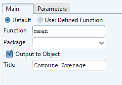
You can also define a new function. To do this select User Defined Function and input function definition on the Definition tab.
The Title section will be used as the name of this module. We named it Compute Average here but you can leave it blank (in that case function name is used as the title).
If the function returns some value, check the Output to Object to let user select the object to assign the returned value. It can be off if the function returns nothing or you do not need to assign the value.
The next step is to add controls to specify arguments of the function. Click on the  button and select x.
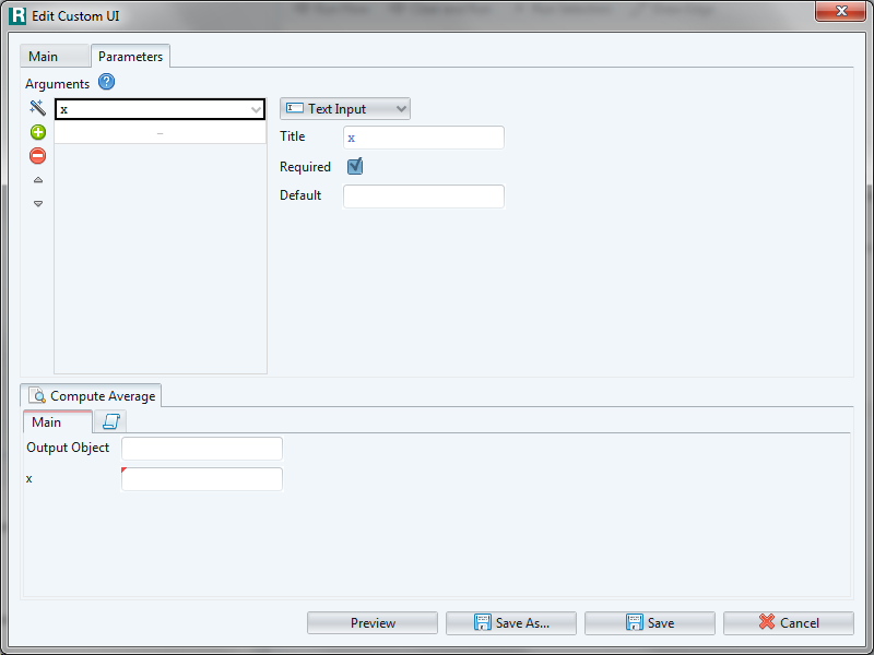
Then an entry is added to the list. You can set a title to this argument but leave it blank for now.
Default is the default value for this argument. But there seems to be no natural default value here, so leave it blank too.
You can check Required to force a user to input some value to this argument. Check it since x cannot be missing for mean function.
The preview is shown below. There are two inputs, Output Object and x. Since x is required it shows an error sign when blank.
Let's add another control about handling NA (Not Available) values. Click on the button again and input na.rm. On the right hand side, select List to add a selection-based control.
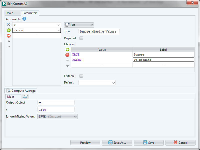
Since the name na.rm may not be meaningful, set Igonre Missing Values as the title.
Tick off the Editable checkbox. If it is on a user can input text instead of select an element, but we do not need this feature here. Leave Default blank.
Then add candidate values for the selection in Choices section. There are two candidates; one is TRUE and put a label Igonre to clarify the meaning of this selection. The other is FALSE with a label Do Nothing.
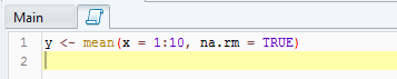
Now review how the new module works. Input some values in the preview area and select the Script tab to review the code generated:
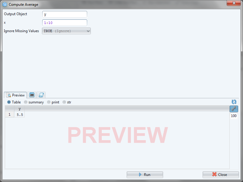
It seems working well. Try clicking on Preview button to test the behavior of this module:
Finally close the test window and click on Save as... button to save this module. It is saved as a .yaml file. Please save it the default directory named custom_ui.
After saving you can access the module from the Custom menu on the toolbar:
Custom modules can also be added to an analysis flow in the same way as built-in modules. Custom nodes can be saved within a flow, so you can send the flow file to other user to let them use these nodes.
You can customize the toolbar to make it preferable for you. For example, you may prefer more space-saving toolbar when working on a small screen.
To change the toolbar settings, click on Preferences > Configuration from the menu and select the Appearance tab.
Version 3.0.4 now works with the latest version of R (3.3.x). This change is required only for Windows; Mac/Linux users can retain the last version (3.0.3).
RAF3 depends on some R packages. However, except for those mentioned in the install process, there is no need to care about them in most cases; you will be asked to install missing packages when needed.
However it becomes a problem when you have only a limited, or no Internet access. For such cases install the packages listed below in advance.
The packages listed below are required:
rJavaJavaGDcodetoolsYou can install all these packages with an R script like below, but please do not try it when RAF is already running:
install.packages(c("rJava", "JavaGD", "codetools"))
Since RAF is dependent on these packages, the installation may fail and can lead to data corruption. As a safer way you can execute it on normal R console before launching RAF, or just launch RAF3 and follow the instructions.
We would like to express appreciation for developers of R and other open source libraries, and FatCow for icons used in RAF3 and this document.
Finally we would also like to acknowledge the contributions from our users. Please mail to rflow-support at ef-prime.com for feedbacks.